Class Meeting 20 (6) Parameterized reports and presentations
100% complete
20.1 Today’s Agenda
- Announcements:
- Firas is away today, Yulia will cover my office hours after lecture in SWNG407
- Hayley Boyce is covering lecture 6 on Parameterized reports
- For cm106 - there is no participation worksheet as it is mostly demos and notes on how to improve your project final report (enjoy the freebie!)
- Next week we will switch gears and (finally) start creating some dashboards using DashR!
- Part 1: Short demos of RMarkdown documents (10 mins)
- RMarkdown presentations
- RMarkdown reports
- Part 2: Output options in RMarkdown (25 mins)
- Review of YAML headers
- Table of contents
- Setting themes
- Output formats (html, md, pdf, word, github)
- Figures and Tables
Break
- Part 3: Parameterized Reports (25 mins)
- Code chunk options (
include,echo,message,warning) - Global options
- How to use R variables in-line with text
- Code chunk options (
- Part 4: Citations in RMarkdown (Optional, if there’s time; 10 mins)
- Bibtex and RMarkdown
- Citing scientific papers
- Citing packages
20.2 Part 1: Short demos of RMarkdown documents
20.2.1 RMarkdown presentations (with citations and references)
20.2.2 RMarkdown reports
20.3 Part 2: YAML Headers and code chunks (25 mins)
First things first, you’ll want the RStudio RMarkdown cheatsheet.
20.3.1 Attribution
This section is adapted from Chapter 2 of Yihui Xie’s book on RMarkdown under a Creative Commons Attribution-NonCommercial-ShareAlike 4.0 International License (CC BY-NC-ND 4.0). Though the sections have been re-arranged, the majority of the content is taken from the textbook directly.
20.3.2 Compile an R Markdown document
The usual way to compile an R Markdown document is to click the Knit button as shown in Figure ??, and the corresponding keyboard shortcut is Ctrl + Shift + K (Cmd + Shift + K on macOS). Under the hood, RStudio calls the function rmarkdown::render() to render the document in a new R session. Please note the emphasis here, which often confuses R Markdown users. Rendering an Rmd document in a new R session means that none of the objects in your current R session (e.g., those you created in your R console) are available to that session.1 Reproducibility is the main reason that RStudio uses a new R session to render your Rmd documents: in most cases, you may want your documents to continue to work the next time you open R, or in other people’s computing environments. See this StackOverflow answer if you want to know more.
If you want to render/knit an Rmd document in a script, you can also call rmarkdown::render() by yourself, and pass the path of the Rmd file to this function. The second argument of this function is the output format, which defaults to the first output format you specify in the YAML metadata (if it is missing, the default is html_document). When you have multiple output formats in the metadata, and do not want to use the first one, you can specify the one you want in the second argument, e.g., for an Rmd document foo.Rmd with the metadata:
You can render it to PDF via:
The function call gives you much more freedom (e.g., you can generate a series of reports in a loop), but you should bear reproducibility in mind when you render documents this way. Of course, you can start a new and clean R session by yourself, and call rmarkdown::render() in that session. As long as you do not manually interact with that session (e.g., manually creating variables in the R console), your reports should be reproducible.
Another main way to work with Rmd documents is the R Markdown Notebooks, which will be introduced in Section 3.2. With notebooks, you can run code chunks individually and see results right inside the RStudio editor. This is a convenient way to interact or experiment with code in an Rmd document, because you do not have to compile the whole document. Without using the notebooks, you can still partially execute code chunks, but the execution only occurs in the R console, and the notebook interface presents results of code chunks right beneath the chunks in the editor, which can be a great advantage. Again, for the sake of reproducibility, you will need to compile the whole document eventually in a clean environment.
Lastly, I want to mention an “unofficial” way to compile Rmd documents: the function xaringan::inf_mr(), or equivalently, the RStudio addin “Infinite Moon Reader”. Obviously, this requires you to install the xaringan package [@R-xaringan], which is available on CRAN. The main advantage of this way is LiveReload: a technology that enables you to live preview the output as soon as you save the source document, and you do not need to hit the Knit button. The other advantage is that it compiles the Rmd document in the current R session, which may or may not be what you desire. Note that this method only works for Rmd documents that output to HTML, including HTML documents and presentations.
A few R Markdown extension packages, such as bookdown and blogdown, have their own way of compiling documents, and we will introduce them later.
Note that it is also possible to render a series of reports instead of single one from a single R Markdown source document. You can parameterize an R Markdown document, and generate different reports using different parameters. See Chapter 15 for details.
20.3.3 Table of contents
You can add a table of contents (TOC) using the toc option and specify the depth of headers that it applies to using the toc_depth option. For example:
If the table of contents depth is not explicitly specified, it defaults to 3 (meaning that all level 1, 2, and 3 headers will be included in the table of contents).
20.3.3.1 Controlling headers/sections in table of contents
The text in an R Markdown document is written with the Markdown syntax. Precisely speaking, it is Pandoc’s Markdown. There are many flavors of Markdown invented by different people, and Pandoc’s flavor is the most comprehensive one to our knowledge. You can find the full documentation of Pandoc’s Markdown at https://pandoc.org/MANUAL.html. We strongly recommend that you read this page at least once to know all the possibilities with Pandoc’s Markdown, even if you will not use all of them. This section is adapted from Section 2.1 of @xie2016, and only covers a small subset of Pandoc’s Markdown syntax.
Section headers can be written after a number of pound signs, e.g.,
If you do not want a certain heading to be numbered, you can add {-} or {.unnumbered} after the heading, e.g.,
20.3.3.2 Floating TOC
You can specify the toc_float option to float the table of contents to the left of the main document content. The floating table of contents will always be visible even when the document is scrolled. For example:
You may optionally specify a list of options for the toc_float parameter which control its behavior. These options include:
collapsed(defaults toTRUE) controls whether the TOC appears with only the top-level (e.g., H2) headers. If collapsed initially, the TOC is automatically expanded inline when necessary.smooth_scroll(defaults toTRUE) controls whether page scrolls are animated when TOC items are navigated to via mouse clicks.
For example:
20.3.4 Setting themes
There are several options that control the appearance of HTML documents:
themespecifies the Bootstrap theme to use for the page (themes are drawn from the Bootswatch theme library). Valid themes include default, cerulean, journal, flatly, darkly, readable, spacelab, united, cosmo, lumen, paper, sandstone, simplex, and yeti. Passnullfor no theme (in this case you can use thecssparameter to add your own styles).highlightspecifies the syntax highlighting style. Supported styles includedefault,tango,pygments,kate,monochrome,espresso,zenburn,haddock,breezedark, andtextmate. Passnullto prevent syntax highlighting.smartindicates whether to produce typographically correct output, converting straight quotes to curly quotes,---to em-dashes,--to en-dashes, and...to ellipses. Note thatsmartis enabled by default.
For example:
20.3.5 Output formats
There are two types of output formats in the rmarkdown package: documents, and presentations. All available formats are listed below:
beamer_presentationcontext_documentgithub_documenthtml_documentioslides_presentationlatex_documentmd_documentodt_documentpdf_documentpowerpoint_presentationrtf_documentslidy_presentationword_document
We will document these output formats in detail in Chapters 3 and 4. There are more output formats provided in other extension packages (described in Chapter 5). For the output format names in the YAML metadata of an Rmd file, you need to include the package name if a format is from an extension package, e.g.,
If the format is from the rmarkdown package, you do not need the rmarkdown:: prefix (although it will not hurt).
When there are multiple output formats in a document, there will be a dropdown menu behind the RStudio Knit button that lists the output format names (Figure 20.1).

Figure 20.1: The output formats listed in the dropdown menu on the RStudio toolbar.
Each output format is often accompanied with several format options. All these options are documented on the R package help pages. For example, you can type ?rmarkdown::html_document in R to open the help page of the html_document format. When you want to use certain options, you have to translate the values from R to YAML, e.g.,
can be written in YAML as:
The translation is often straightforward. Remember that R’s TRUE, FALSE, and NULL are true, false, and null, respectively, in YAML. Character strings in YAML often do not require the quotes (e.g., dev: 'svg' and dev: svg are the same), unless they contain special characters, such as the colon :.
If a certain option has sub-options (which means the value of this option is a list in R), the sub-options need to be further indented, e.g.,
Some options are passed to knitr, such as dev, fig_width, and fig_height. Detailed documentation of these options can be found on the knitr documentation page: https://yihui.name/knitr/options/. Note that the actual knitr option names can be different. In particular, knitr uses . in names, but rmarkdown uses _, e.g., fig_width in rmarkdown corresponds to fig.width in knitr. We apologize for the inconsistencies—programmers often strive for consistencies in their own world, yet one standard plus one standard often equals three standards. If I were to design the knitr package again, I would definitely use _.
20.3.6 Figures and Tables
Here are some notes on how to control figure captions, width, height etc…
fig.widthandfig.height: The (graphical device) size of R plots in inches. R plots in code chunks are first recorded via a graphical device in knitr, and then written out to files. You can also specify the two options together in a single chunk optionfig.dim, e.g.,fig.dim = c(6, 4)meansfig.width = 6andfig.height = 4.out.widthandout.height: The output size of R plots in the output document. These options may scale images. You can use percentages, e.g.,out.width = '80%'means 80% of the page width.fig.align: The alignment of plots. It can be'left','center', or'right'.
By default, figures produced by R code will be placed immediately after the code chunk they were generated from. For example:
You can provide a figure caption using fig.cap in the chunk options. If the document output format supports the option fig_caption: true (e.g., the output format rmarkdown::html_document), the R plots will be placed into figure environments. In the case of PDF output, such figures will be automatically numbered. If you also want to number figures in other formats (such as HTML), please see the bookdown package in Chapter 12.
PDF documents are generated through the LaTeX files generated from R Markdown. A highly surprising fact to LaTeX beginners is that figures float by default: even if you generate a plot in a code chunk on the first page, the whole figure environment may float to the next page. This is just how LaTeX works by default. It has a tendency to float figures to the top or bottom of pages. Although it can be annoying and distracting, we recommend that you refrain from playing the “Whac-A-Mole” game in the beginning of your writing, i.e., desparately trying to position figures “correctly” while they seem to be always dodging you. You may wish to fine-tune the positions once the content is complete using the fig.pos chunk option (e.g., fig.pos = 'h'). See https://www.overleaf.com/learn/latex/Positioning_images_and_tables for possible values of fig.pos and more general tips about this behavior in LaTeX. In short, this can be a difficult problem for PDF output.
To place multiple figures side-by-side from the same code chunk, you can use the fig.show='hold' option along with the out.width option. Figure ?? shows an example with two plots, each with a width of 50%.
ggplot(mtcars, aes(factor(cyl), fill = factor(vs))) +
  geom_bar(position = position_dodge2(preserve = "single")) + theme_bw()

ggplot(mtcars, aes(factor(cyl), fill = factor(vs))) +
  geom_bar(position = position_dodge2(preserve = "total")) + theme_bw()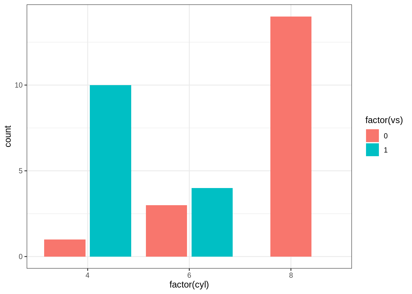
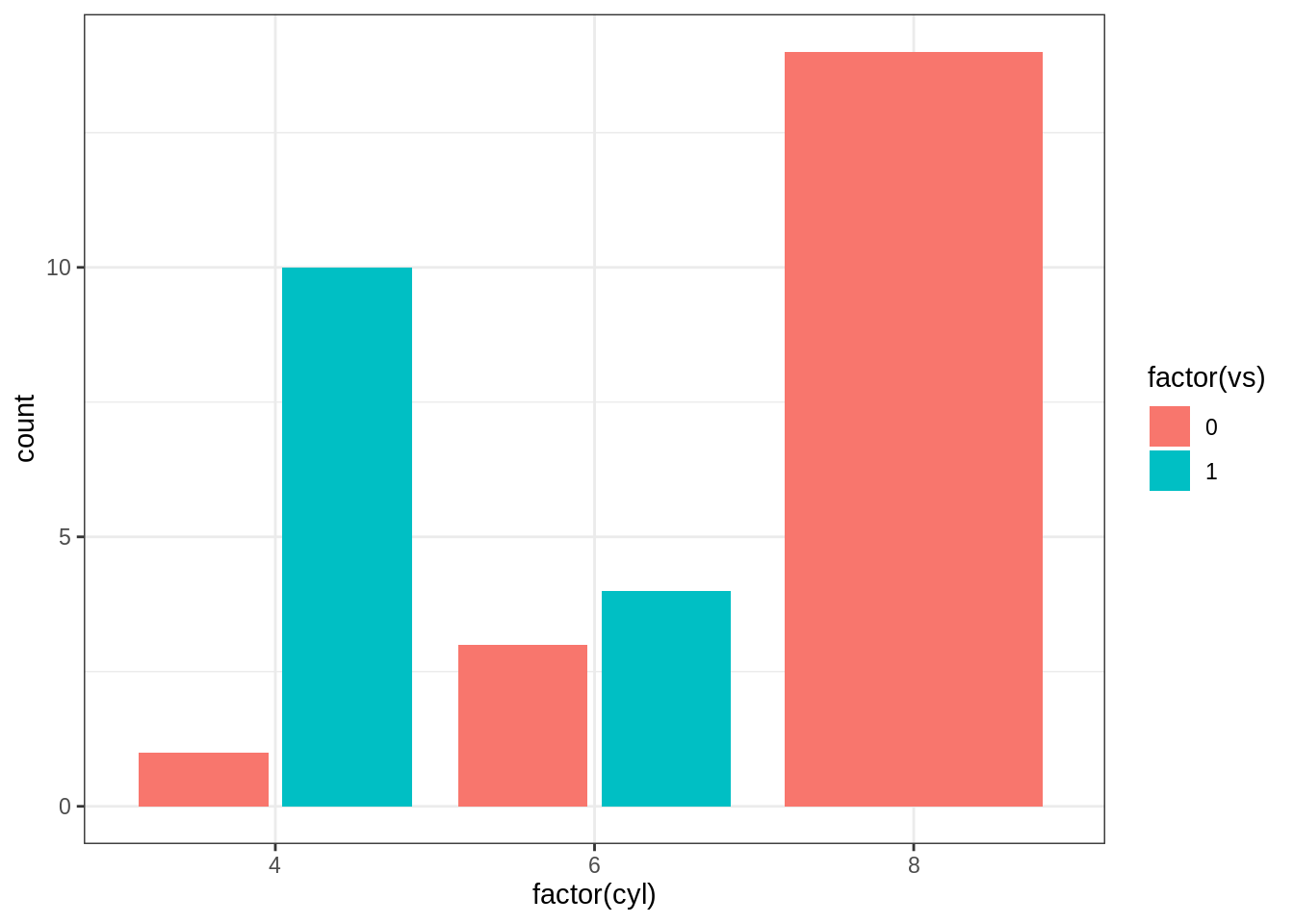
Figure 20.2: Two plots side-by-side.
Of course, you could also just use the plot_grid function from the cowplots package - which is a much more powerful option.
If you want to include a graphic that is not generated from R code, you may use the knitr::include_graphics() function, which gives you more control over the attributes of the image than the Markdown syntax of  (e.g., you can specify the image width via out.width). Figure 20.3 provides an example of this.
```{r, out.width='25%', fig.align='center', fig.cap='...'}
knitr::include_graphics('https://github.com/rstudio/rmarkdown-book/raw/master/images/hex-rmarkdown.png')
```
Figure 20.3: The R Markdown hex logo.
20.4 Part 3: Parameterized reporting (25 mins)
20.4.1 Code chunk options (include, echo, message, warning)
You can insert an R code chunk either using the RStudio toolbar (the Insert button) or the keyboard shortcut Ctrl + Alt + I (Cmd + Option + I on macOS).
There are a lot of things you can do in a code chunk: you can produce text output, tables, or graphics. You have fine control over all these output via chunk options, which can be provided inside the curly braces (between ```{r and }). For example, you can choose hide text output via the chunk option results = 'hide', or set the figure height to 4 inches via fig.height = 4. Chunk options are separated by commas, e.g.,
The value of a chunk option can be an arbitrary R expression, which makes chunk options extremely flexible. For example, the chunk option eval controls whether to evaluate (execute) a code chunk, and you may conditionally evaluate a chunk via a variable defined previously, e.g.,
```{r}
# execute code if the date is later than a specified day
do_it = Sys.Date() > '2018-02-14'
```

```{r, eval=do_it}
x = rnorm(100)
```
There are a large number of chunk options in knitr documented at https://yihui.name/knitr/options. We list a subset of them below:
eval: Whether to evaluate a code chunk.echo: Whether to echo the source code in the output document. This is useful if you want to show just your results and hide your source code.results: When set to'hide', text output will be hidden; when set to'asis', text output is written “as-is”, e.g., you can write out raw Markdown text from R code (likecat('**Markdown** is cool.\n')). By default, text output will be wrapped in verbatim elements (typically plain code blocks).collapse: Whether to merge text output and source code into a single code block in the output. This is mostly cosmetic:collapse = TRUEmakes the output more compact, since the R source code and its text output are displayed in a single output block. The defaultcollapse = FALSEmeans R expressions and their text output are separated into different blocks.warning,message, anderror: Whether to show warnings, messages, and errors in the output document. Note that if you seterror = FALSE,rmarkdown::render()will halt on error in a code chunk, and the error will be displayed in the R console. Similarly, whenwarning = FALSEormessage = FALSE, these messages will be shown in the R console.include: Whether to include anything from a code chunk in the output document. Wheninclude = FALSE, this whole code chunk is excluded in the output, but note that it will still be evaluated ifeval = TRUE. When you are trying to setecho = FALSE,results = 'hide',warning = FALSE, andmessage = FALSE, chances are you simply mean a single optioninclude = FALSEinstead of suppressing different types of text output individually.fig.cap: The figure caption.
There is an optional chunk option that does not take any value, which is the chunk label. It should be the first option in the chunk header. Chunk labels are mainly used in filenames of plots and cache. If the label of a chunk is missing, a default one of the form unnamed-chunk-i will be generated, where i is incremental. I strongly recommend that you only use alphanumeric characters (a-z, A-Z and 0-9) and dashes (-) in labels, because they are not special characters and will surely work for all output formats. Other characters may cause trouble in certain packages, such as bookdown.
20.4.2 Global options
If a certain option needs to be frequently set to a value in multiple code chunks, you can consider setting it globally in the first code chunk of your document, e.g.,
20.4.3 How to use R variables in-line with text
Besides code chunks, you can also insert values of R objects inline in text. For example:
For a circle with the radius 5, its area is 78.5398163.
When you knit this file, the above should do a calculation that computes the Area of a circle with radius r=5.
This is perhaps one of the coolest features of RMarkdown! You should definitely use this feature in your STAT 547 project! There are many ways this can be useful, including reporting of summary statistics, or reporting on your linear regression, etc…
20.5 OPTIONAL Part 4: Citations and Cross-references in RMarkdown (10 mins)
There are multiple ways to insert citations, and we recommend that you use BibTeX databases, because they work better when the output format is LaTeX/PDF. Section 2.8 of @xie2016 has explained the details. The key idea is that when you have a BibTeX database (a plain-text file with the conventional filename extension .bib) that contains entries like:
@Manual{R-base,
  title = {R: A Language and Environment for Statistical
    Computing},
  author = {{R Core Team}},
  organization = {R Foundation for Statistical Computing},
  address = {Vienna, Austria},
  year = {2017},
  url = {https://www.R-project.org/},
}
Note: Thisfollowing paragraphs are from the bookdown textbook Section 2.8 used under a Creative Commons Attribution-NonCommercial-ShareAlike 4.0 International License (CC BY-NC-ND 4.0).
A bibliography entry starts with @type{, where type may be article, book, manual, and so on.2 Then there is a citation key, like R-base in the above example. To cite an entry, use @key or [@key] (the latter puts the citation in braces), e.g., @R-base is rendered as @R-base, and [@R-base] generates “[@R-base]”. If you are familiar with the natbib package in LaTeX, @key is basically \citet{key}, and [@key] is equivalent to \citep{key}.
There are a number of fields in a bibliography entry, such as title, author, and year, etc. You may see https://en.wikipedia.org/wiki/BibTeX for possible types of entries and fields in BibTeX.
There is a helper function write_bib() in knitr to generate BibTeX entries automatically for R packages. Note that it only generates one BibTeX entry for the package itself at the moment, whereas a package may contain multiple entries in the CITATION file, and some entries are about the publications related to the package. These entries are ignored by write_bib().
@Manual{R-knitr,
  title = {knitr: A General-Purpose Package for Dynamic Report
    Generation in R},
  author = {Yihui Xie},
  year = {2020},
  note = {R package version 1.28},
  url = {https://CRAN.R-project.org/package=knitr},
}
@Manual{R-stringr,
  title = {stringr: Simple, Consistent Wrappers for Common
    String Operations},
  author = {Hadley Wickham},
  year = {2019},
  note = {R package version 1.4.0},
  url = {https://CRAN.R-project.org/package=stringr},
}
@Book{knitr2015,
  title = {Dynamic Documents with {R} and knitr},
  author = {Yihui Xie},
  publisher = {Chapman and Hall/CRC},
  address = {Boca Raton, Florida},
  year = {2015},
  edition = {2nd},
  note = {ISBN 978-1498716963},
  url = {https://yihui.org/knitr/},
}
@InCollection{knitr2014,
  booktitle = {Implementing Reproducible Computational
    Research},
  editor = {Victoria Stodden and Friedrich Leisch and Roger D.
    Peng},
  title = {knitr: A Comprehensive Tool for Reproducible
    Research in {R}},
  author = {Yihui Xie},
  publisher = {Chapman and Hall/CRC},
  year = {2014},
  note = {ISBN 978-1466561595},
  url = {http://www.crcpress.com/product/isbn/9781466561595},
}
Once you have one or multiple .bib files, you may use the field bibliography in the YAML metadata of your first R Markdown document (which is typically index.Rmd), and you can also specify the bibliography style via biblio-style (this only applies to PDF output), e.g.,
---
bibliography: ["one.bib", "another.bib", "yet-another.bib"]
biblio-style: "apalike"
link-citations: true
---
The field link-citations can be used to add internal links from the citation text of the author-year style to the bibliography entry in the HTML output.
When the output format is LaTeX, citations will be automatically put in a chapter or section. For non-LaTeX output, you can add an empty chapter as the last chapter of your book. For example, if your last chapter is the Rmd file 06-references.Rmd, its content can be an inline R expression:
You may add a field named bibliography to the YAML metadata, and set its value to the path of the BibTeX file. Then in Markdown, you may use @R-base (which generates “@R-base”) or [@R-base] (which generates “[@R-base]”) to reference the BibTeX entry. Pandoc will automatically generated a list of references in the end of the document.
20.5.1 Cross-referencing
You can also reference sections using the same syntax \@ref(label), where label is the section ID. By default, Pandoc will generate an ID for all section headers, e.g., a section # Hello World will have an ID hello-world. We recommend you to manually assign an ID to a section header to make sure you do not forget to update the reference label after you change the section header. To assign an ID to a section header, simply add {#id} to the end of the section header. Further attributes of section headers can be set using standard Pandoc syntax.
When a referenced label cannot be found, you will see two question marks like ??, as well as a warning message in the R console when rendering the book.
You can also create text-based links using explicit or automatic section IDs or even the actual section header text.
- If you are happy with the section header as the link text, use it inside a single set of square brackets:
- [Section header text]: example “[A single document]” via [A single document]
- There are two ways to specify custom link text:
- [link text][Section header text], e.g., “[non-English books][Internationalization]” via [non-English books][Internationalization]
- [link text](#ID), e.g., “Table stuff” via [Table stuff](#tables)
The Pandoc documentation provides more details on automatic section IDs and implicit header references.
Cross-references still work even when we refer to an item that is not on the current page of the PDF or HTML output.
20.6 Take-home messages
- RMarkdown is incredibly powerful and gives you many, many options for creating reports, presentations, documents, analysis notebooks!
- Understanding YAML headers and all the different knitr options will really help you leverage RMarkdown reports
- You can easily turn your RMarkdown reports into beautiful presentations!
- More advanced usage of RMarkdown documents includes using cross-references and citations (use these to stay organized)
- Adding in-line R-code to your RMarkdown documents will change your life; I encourage you to add these to your report so you at least have a example of how they work!