Class Meeting 12 Working with factors in R
Today’s class is working with a very important component of R - factors.
12.1 Worksheet
Link to cm012 worksheet file.
12.2 Resources
12.2.1 References and tutorials
- Jenny Bryan’s notes on factors
12.2.2 Package documentation
- forcats package
Load the required libraries. You might need to install library forcats first (install.packages(“forcats”))
12.3 Recap of CM011
Outline of last lecture lecture
- here package
- read/write_csv (and friends)
- read_excel() function from readxl package
- data processing and importing
12.4 Motivating the need for factors in R
12.4.1 Activity 1: Using Factors for plotting
1.1 Let’s look again into gapminder dataset and create a new cloumn, life_level, that contains five categories (“very high”, “high”,“moderate”, “low” and “very low”) based on life expectancy in 1997. Assign categories accoring to the table below:
| Criteria | life_level |
|---|---|
| less than 23 | very low |
| between 23 and 48 | low |
| between 48 and 59 | moderate |
| between 59 and 70 | high |
| more than 70 | very high |
Function case_when() is a tidier way to vectorise multiple if_else() statements. you can read more about this function here.
gapminder %>%
  filter(year == 1997) %>%
  mutate(life_level = case_when(lifeExp < 23 ~ 'very low',
                                lifeExp < 48~ 'low',
                                lifeExp < 59 ~ 'moderate',
                                lifeExp < 70 ~ 'high',
                                TRUE ~ 'very high')) %>%
  ggplot() + geom_boxplot(aes(x = life_level, y = gdpPercap)) +
  labs(y = "GDP per capita, $", x= "Life expectancy level, years") +
theme_bw() 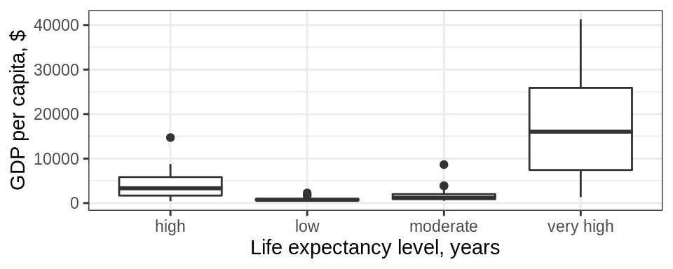
Do you notice anything odd/wrong about the graph?
We can make a few observations:
It seems that none of the countries had a “very low” life-expectancy in 1997.
However, since it was an option in our analysis it should be included in our plot. Right?
Notice also how levels on x-axis are placed in the “wrong” order.
1.2 You can correct these issues by explicitly setting the levels parameter in the call to factor(). Use, drop = FALSE to tell the plot not to drop unused levels
gapminder %>%
  filter(year == 1997) %>%
  mutate(life_level = factor(case_when(lifeExp < 23 ~ 'very low',
                                lifeExp < 48~ 'low',
                                lifeExp < 59 ~ 'moderate',
                                lifeExp < 70 ~ 'high',
                                TRUE ~ 'very high'),
                levels = c("very low" , "low","moderate", "high","very high"))) %>%
  ggplot() + geom_boxplot(aes(x = life_level, y = gdpPercap)) +
  labs(y = "GDP per capita, $", x= "Life expectancy level, years") +
  theme_bw() +
  scale_x_discrete(drop = FALSE)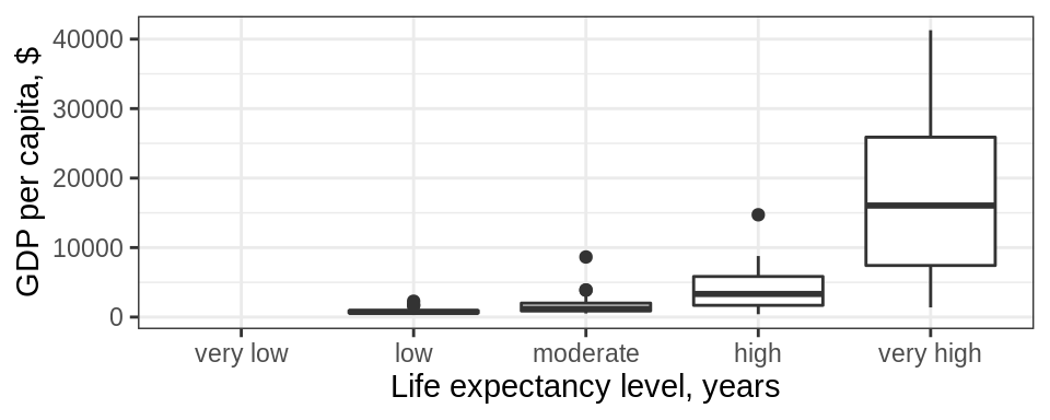
12.5 Inspecting factors (activity 2)
In Activity 1, we created our own factors, so now let’s explore what categorical variables that we have in the gapminder dataset.
12.5.1 Exploring gapminder$continent (activity 2.1)
Use functions such as str(), levels(), nlevels() and class() to answer the following questions:
- what class is
continent(a factor or charecter)? - How many levels? What are they?
- What integer is used to represent factor “Asia”?
## [1] "factor"## [1] "Africa" "Americas" "Asia" "Europe" "Oceania"## [1] 5## Factor w/ 5 levels "Africa","Americas",..: 3 3 3 3 3 3 3 3 3 3 ...## # A tibble: 1,704 x 6
## country continent year lifeExp pop gdpPercap
## <fct> <fct> <int> <dbl> <int> <dbl>
## 1 Afghanistan Asia 1952 28.8 8425333 779.
## 2 Afghanistan Asia 1957 30.3 9240934 821.
## 3 Afghanistan Asia 1962 32.0 10267083 853.
## 4 Afghanistan Asia 1967 34.0 11537966 836.
## 5 Afghanistan Asia 1972 36.1 13079460 740.
## 6 Afghanistan Asia 1977 38.4 14880372 786.
## 7 Afghanistan Asia 1982 39.9 12881816 978.
## 8 Afghanistan Asia 1987 40.8 13867957 852.
## 9 Afghanistan Asia 1992 41.7 16317921 649.
## 10 Afghanistan Asia 1997 41.8 22227415 635.
## # … with 1,694 more rows12.5.2 Exploring gapminder$country (activity 2.2)
Let’s explore what else we can do with factors:
Answer the following questions:
- How many levels are there in
country? - Filter
gapminderdataset by 5 countries of your choice. How many levels are in your filtered dataset?
## [1] 142h_countries <- c("Egypt", "Haiti", "Romania", "Thailand", "Venezuela")
h_gap <- gapminder %>%
filter(country %in% h_countries)
nlevels(h_gap$country)## [1] 14212.6 Dropping unused levels
What if we want to get rid of some levels that are “unused” - how do we do that?
The function droplevels() operates on all the factors in a data frame or on a single factor. The function forcats::fct_drop() operates on a factor.
## [1] 512.7 Changing the order of levels
Let’s say we wanted to re-order the levels of a factor using a new metric - say, count().
We should first produce a frequency table as a tibble using dplyr::count():
## # A tibble: 5 x 2
##   continent     n
##   <fct>     <int>
## 1 Africa      624
## 2 Americas    300
## 3 Asia        396
## 4 Europe      360
## 5 Oceania      24
The table is nice, but it would be better to visualize the data. Factors are most useful/helpful when plotting data. So let’s first plot this:
gapminder %>%
  ggplot() +
  geom_bar(aes(continent)) +
  coord_flip()+
  theme_bw() +
  ylab("Number of entries") + xlab("Continent")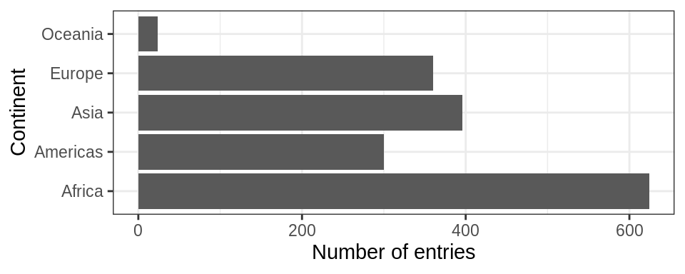
Think about how levels are normally ordered. It turns out that by default, R always sorts levels in alphabetical order. However, it is preferable to order the levels according to some principle:
- Frequency/count.
- Make the most common level the first and so on. Function
fct_infreq()might be useful. - The function
fct_rev()will sort them in the opposite order.
For instance , `
gapminder %>%
  ggplot() +
  geom_bar(aes(fct_infreq(continent))) +
  coord_flip()+
  theme_bw() +
  ylab("Number of entries") + xlab("Continent")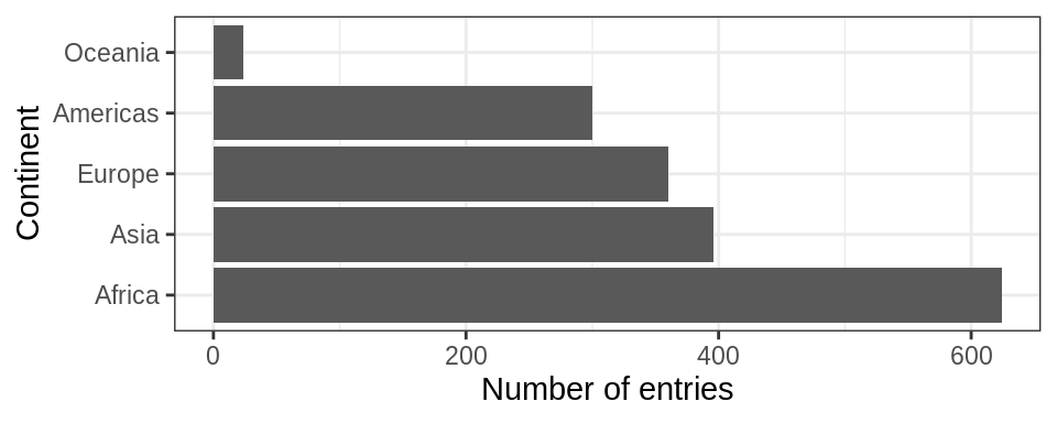
Section 9.6 of Jenny Bryan’s notes has some helpful examples.
- Another variable.
- For example, if we wanted to bring back our example of ordering
gapmindercountries by life expectancy, we can visualize the results usingfct_reorder().
##  default summarizing function is median()
gapminder %>%
  ggplot() +
  geom_bar(aes(fct_reorder(continent, lifeExp, max))) +
  coord_flip()+
  theme_bw() +
xlab("Continent")+ylab("Number of entries") 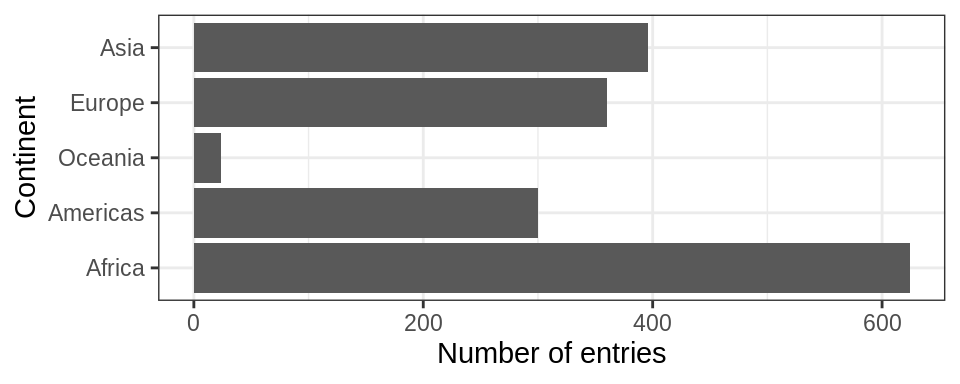
Use fct_reorder2() when you have a line chart of a quantitative x against another quantitative y and your factor provides the color.
## order by life expectancy
ggplot(h_gap, aes(x = year, y = lifeExp,
                  color = fct_reorder2(country, year, lifeExp))) +
  geom_line() +
  labs(color = "country")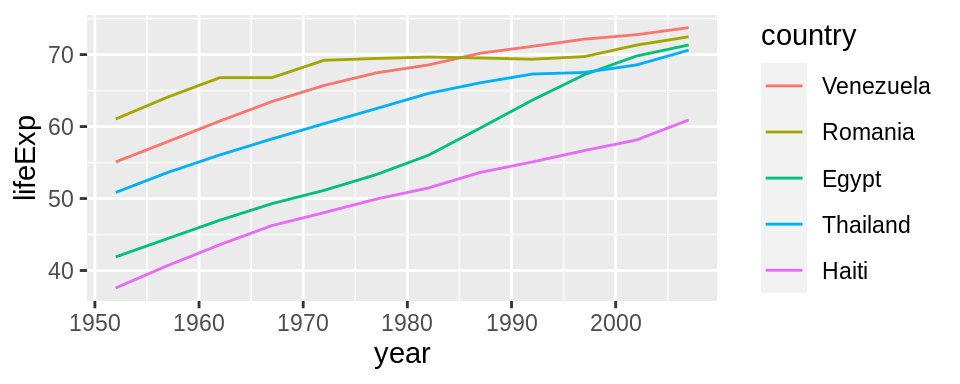
12.8 Change order of the levels manually
This might be useful if you are preparing a report for say, the state of affairs in Africa.
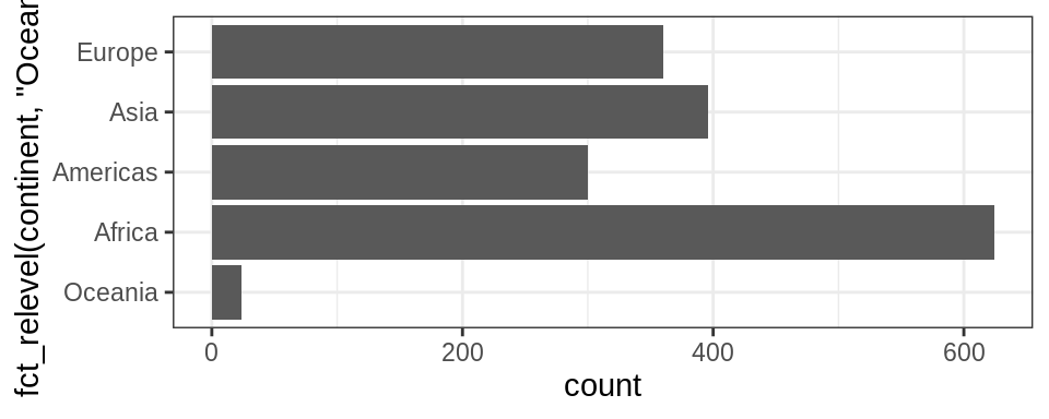 More details on reordering factor levels by hand can be found [here] https://forcats.tidyverse.org/reference/fct_relevel.html
12.8.1 Recoding factors
Sometimes you want to specify what the levels of a factor should be.
For instance, if you had levels called “blk” and “brwn”, you would rather they be called “Black” and “Brown” - this is called recoding.
Lets recode Oceania and the Americas in the graph above as abbreviations OCN and AME respectively using the function fct_recode().
gapminder %>%
  ggplot() +
  geom_bar(aes(fct_recode(continent,"OCN"="Oceania" , "AME" = "Americas"))) +
  coord_flip()+
  theme_bw()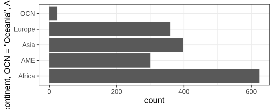
12.9 Grow a factor (OPTIONAL)
Let’s create two data frames,df1 and df2 each with data from two countries, dropping unused factor levels.
df1 <- gapminder %>%
  filter(country %in% c("United States", "Mexico"), year > 2000) %>%
  droplevels()
df2 <- gapminder %>%
  filter(country %in% c("France", "Germany"), year > 2000) %>%
  droplevels()
The country factors in df1 and df2 have different levels. Can we just combine them?
## [1] 1 1 2 2 1 1 2 2The country factors in df1 and df2 have different levels.
Can you just combine them using c()?
## [1] Mexico        Mexico        United States United States France
## [6] France        Germany       Germany
## Levels: Mexico United States France Germany
Explore how different forms of row binding work behave here, in terms of the country variable in the result.
## Warning in bind_rows_(x, .id): Unequal factor levels: coercing to character## Warning in bind_rows_(x, .id): binding character and factor vector, coercing
## into character vector
## Warning in bind_rows_(x, .id): binding character and factor vector, coercing
## into character vector## Warning in bind_rows_(x, .id): Unequal factor levels: coercing to character## Warning in bind_rows_(x, .id): binding character and factor vector, coercing
## into character vector
## Warning in bind_rows_(x, .id): binding character and factor vector, coercing
## into character vector## # A tibble: 8 x 6
## country continent year lifeExp pop gdpPercap
## <chr> <chr> <int> <dbl> <int> <dbl>
## 1 Mexico Americas 2002 74.9 102479927 10742.
## 2 Mexico Americas 2007 76.2 108700891 11978.
## 3 United States Americas 2002 77.3 287675526 39097.
## 4 United States Americas 2007 78.2 301139947 42952.
## 5 France Europe 2002 79.6 59925035 28926.
## 6 France Europe 2007 80.7 61083916 30470.
## 7 Germany Europe 2002 78.7 82350671 30036.
## 8 Germany Europe 2007 79.4 82400996 32170.## # A tibble: 8 x 6
## country continent year lifeExp pop gdpPercap
## <fct> <fct> <int> <dbl> <int> <dbl>
## 1 Mexico Americas 2002 74.9 102479927 10742.
## 2 Mexico Americas 2007 76.2 108700891 11978.
## 3 United States Americas 2002 77.3 287675526 39097.
## 4 United States Americas 2007 78.2 301139947 42952.
## 5 France Europe 2002 79.6 59925035 28926.
## 6 France Europe 2007 80.7 61083916 30470.
## 7 Germany Europe 2002 78.7 82350671 30036.
## 8 Germany Europe 2007 79.4 82400996 32170.